Dynamic Scripting Workflow

coRps Session on Dynamic Scripting Workflow

Overview

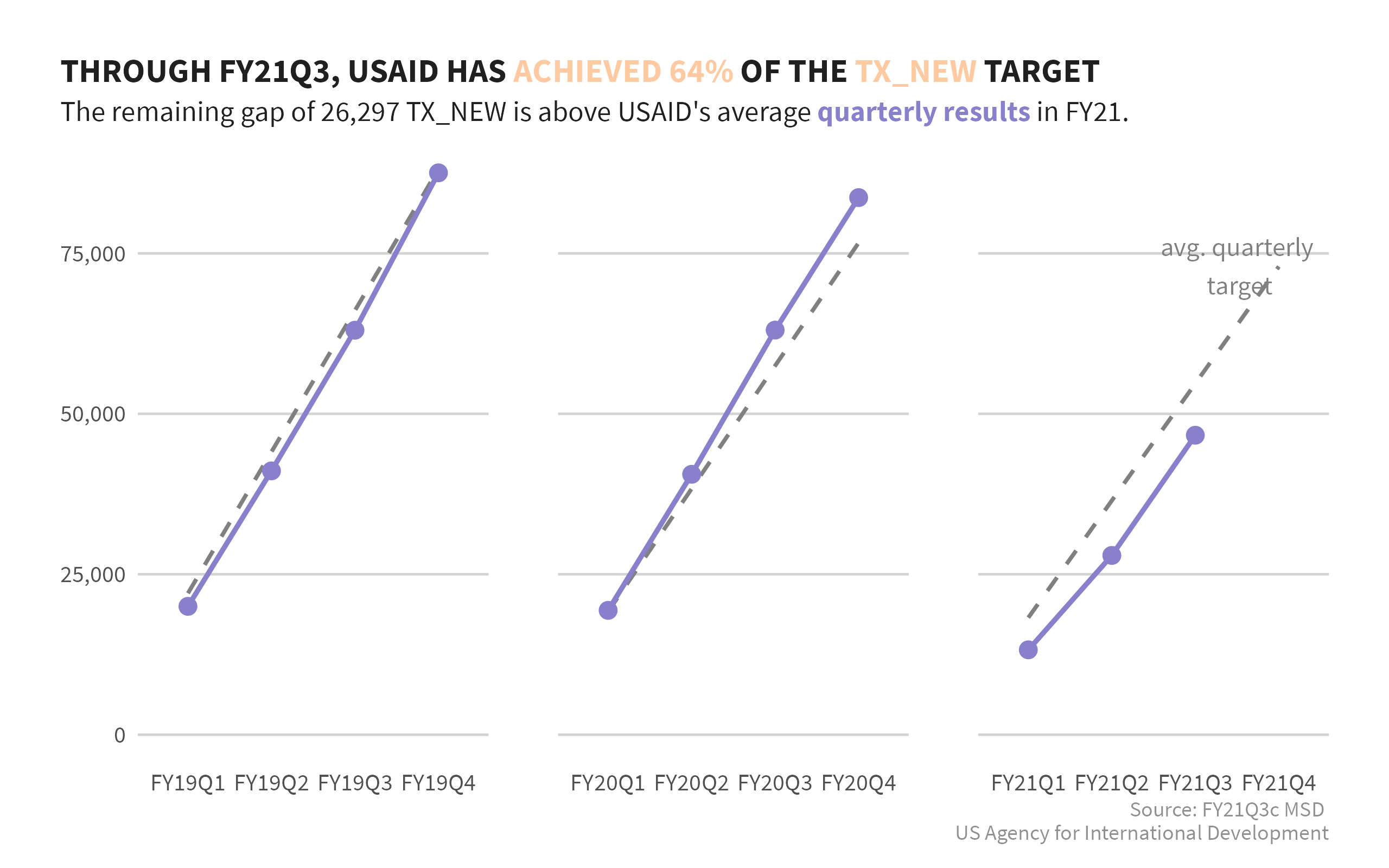
Our goal today is to see how we can be more dynamic in our code, allowing for automation of our workflows and decreasing the time it takes to update munging, analysis, or visualization each time your data are refreshed. With that in mind, we’ll walk through a typical workflow. Our work will be guided by answering the following question: is USAID/Tanzania on track to reaching it’s FY21 TX_NEW targets and how does this compare to prior years?

Packages

Let’s start by load our standard set of packages for munging and plotting MER data. Packages like glitr, glamr, and gophr are USAID/OHA custom packages.

  library(tidyverse)
  library(glitr)  #remotes::install_github("USAID-OHA-SI/glitr", build_vignettes = TRUE)
  library(glamr)  #remotes::install_github("USAID-OHA-SI/glamr", build_vignettes = TRUE)
  library(gophr)  #remotes::install_github("USAID-OHA-SI/gohpr", build_vignettes = TRUE)
  library(extrafont)
  library(scales)
  library(ggtext)
  library(glue)

Download MSD

We’ll need the OUxIM MSD for this exercise. You can manually download it from PEPFAR Panorama or follow the steps in the glamr vignette, called “Data Extraction from Panorama”. We won’t have time to walk through the download automation today, but this is a super great resource added in FY21Q3.

Access most recent MSD

Given the size of the MER Strutured Datasets (MSDs), we typically store the most recent files in a central folder locally rather than having each project folder having it’s own separate set of MSD files. Since my folder location for the data will be different than you’re we’ve creates a way for you to store the folder path in your .Rprofile so that we can all run the same code without having to manually change anything. If you don’t have your MSD folder path saved, you can use set_paths() like below to store your path

set_paths(folderpath_msd = "C:/Users/spower/Documents/Data")

Now that you have the path stored, you can utilize this in combination with glamr::return_latest(), to return the latest file (the MSD) that matches a specific pattern. In this case, we want the OUxIM FY19-22 dataset. And then lastly, we can read in the file using gophr::read_msd() (the first time you download the file, you should convert it to a compressed .rds file to take up less space - read_msd(path, save_rds = TRUE, remove_txt = TRUE)).

df <- si_path() %>% 
  return_latest("OU_IM_FY19") %>% 
  read_msd()   

Munge

The MSD is loaded into our R session so we can start using it. We’re going to start by specifying the indicator we want to work with as an object, allowing us to use it in multiple places in our analysis and make it easier to update if needed.

ind_sel <- "TX_NEW"

To answer the question, we need to limit our dataset down to just USAID/Tanzania for TX_NEW. We only need the total numerator and we’ll aggregate this up to by fiscal year. I’ve also included the indicator in the group_by() since we’ll need it to preform our quarterly reshape (the function needs to know the indicator to then know if it should use a snapshot or cumulative value when creating the cumulative sum).

df_tza <- df %>% 
  filter(operatingunit == "Tanzania",
         fundingagency == "USAID",
         indicator == ind_sel,
         standardizeddisaggregate == "Total Numerator") %>% 
  group_by(fiscal_year, indicator) %>% 
  summarise(across(c("targets", starts_with("qtr")), sum, na.rm = TRUE),
            .groups = "drop")

The reshape will drop future periods, but we want to keep anything in the current FY for our plot, so we give any quarter in the current FY a negative value to keep it (it will drop if its zero). We need to know the current fiscal year, so we call pull that using glamr::source_info(), which uses information from the file name to know the current period.

(curr_fy <- source_info(return = "fiscal_year"))

## [1] 2021

df_tza <- df_tza %>%
  mutate(across(starts_with("qtr"), 
                ~ ifelse(. == 0 & fiscal_year == curr_fy, -1, .))) %>% 
  reshape_msd("quarters", qtrs_keep_cumulative = TRUE) %>% 
  mutate(results = na_if(results, -1),
         results_cumulative = ifelse(is.na(results), NA, results_cumulative))

In our plot we want to track cumulative quarterly achievement against an estimated quarterly target, so we need to extract the quarter from the period and use that to calcuate the quarterly target. We’ll also add annotation text to label this in the plot.

df_tza <- df_tza %>% 
  adorn_achievement() %>% 
  group_by(fiscal_year) %>% 
  mutate(qtr = str_sub(period, -1) %>% as.numeric,
         targets_qtrly = targets * (qtr/4)) %>% 
  ungroup() %>% 
  mutate(anno_lab = case_when(period == max(period) ~ "avg. quarterly\n target"))

We used source_info() earlier to get the year, but we will now use it to get other information so we can make our text dynamic in the plot. We’ll also create a data frame (curr_achv) that has information that will be included in the plot, rather than manually editing the information.

(msd_source <- source_info())

## FY21Q3c MSD

(curr_pd <- source_info(return = "period"))

## FY21Q3

curr_achv <- df_tza %>% 
  filter(fiscal_year == curr_fy) %>% 
  mutate(avg = mean(results, na.rm = TRUE),
         gap = targets - results_cumulative,
         gap_qtrly = gap / (4 - qtr),
         direction = ifelse(avg > gap_qtrly, "less than", "above")) %>% 
  filter(period == curr_pd)

Alright, now it’s time to plot. We are plotting cumulative results by period as well as the quarterly targets. We’ve added in the annotation to the current fiscal year’s Q4 point. Most of the dyanmic text is occurring in the title and caption.

df_tza %>% 
  ggplot(aes(period, results_cumulative, group = fiscal_year)) +
  geom_line(aes(y = targets_qtrly), color = trolley_grey, size = .8, linetype = "dashed") +
  geom_line(size = 1, color = moody_blue, na.rm = TRUE) +
  geom_point(size = 3, color = moody_blue, na.rm = TRUE) +
  geom_text(aes(y = targets_qtrly, label = anno_lab), na.rm = TRUE,
            family = "Source Sans Pro", color = trolley_grey, nudge_x = -.5) +
  facet_grid(~ fiscal_year, scales = "free_x") +
  expand_limits(y = 0) +
  scale_y_continuous(labels = comma) +
  labs(x = NULL, y = NULL,
       title = glue("THROUGH {curr_pd}, USAID HAS <span style = 'color:{curr_achv$achv_color};'>ACHIEVED {percent(curr_achv$achievement_qtrly, 1)}</span> OF THE <span style = 'color:{curr_achv$achv_color};'>{ind_sel} </span>TARGET"),
       subtitle = glue("The remaining gap of {comma(curr_achv$gap, 1)} {ind_sel} is {curr_achv$direction} USAID's average **<span style = 'color:{moody_blue};'>quarterly results </span>**in {str_sub(curr_pd, end = 4)}."),
       caption = glue("Source: {msd_source} 
                      US Agency for International Development")) +
  si_style_ygrid() +
  theme(strip.text.x = element_blank(),
        plot.title = element_markdown(),
        plot.subtitle = element_markdown())

Take a look over the code and compare that with the plot. If we ran this again next quarter, we wouldn’t have to change anything at all. If we wanted to look at HTS_TST_POS instead, we can swap that out at the very tope and just rerun the code, no need to hunt for each place you used the static text.

Structuring your code in this way might take a bit more work to think through when you get started, but it makes your code much more robust, transparent, and reproducible.