RBBS - 6 Importing Data
2022-03-28 Aaron Chafetz
corps rbbs r
Part 6 of the coRps R Building Blocks Series (RBBS). All content can be found on this blog under the rbbs category as well as on the USAID-OHA-SI/coRps GitHub repo.
RBBS 6 - Importing Data
For our R Building Blocks session today, we covering different methods
and parameters for importing data into R. This session covers much of
the content found in Chapter 11 of R for Data
Science and focuses on using
the readr package.
Learning Objectives
- Know what different packages exist to read in data and when to use them
- Understand key parameters useful across different packages
- Develop an approach to reviewing and knowing how to import data
Recording
USAID staff can use this link to access today’s recording (not available to external users).
Materials
Setup
For these sessions, we’ll be using RStudio which is an IDE, “Integrated development environment” that makes it easier to work with R. For help on getting setup and installing packages, please reference this guide.
Introduction
Over the last few sessions, we’ve covered the principles of tidy
data
and gone over key functions to work with data in base R and the
tidyverse.
Before you can really apply these tools, you have to be able to know how
to bring data into R. If we look at the graphic from the last session,
we can see that import is the first step in our data exploration journey
and we will rely heavily on readr, but we will also cover some other
tools along the way.
A quick aside as well, in our office as is true many places, the default way of sharing data is often in Excel spreadsheets. When it comes to R and most stats packages and programming languages, we can read in Excel sheets, but the preference is to use csv files, where csv stands for comma separated value, since they:
- do not need a specific platform or software to open;
- are faster, less complicated (no user formatting stored); and
- typically consumes less memory.
Load packages
library(tidyverse) #install.packages("tidyverse"); contains readr and purrr
library(readxl) #install.packages("readxl")
library(googlesheets4) #install.packages("googlesheets4")
library(vroom) #install.packages("vroom")
library(gophr) #remotes::install_github("USAID-OHA-SI/gophr", build_vignettes = TRUE)
Reading in data
Let’s start by reading in a basic csv file. The best first step when reading in any file is to inspect it first to understand its structure and any possible complications. Since this the file is a csv, you can preview it in a text editor or open it up in Excel. Let’s open up this file (simple.csv) and review it contents.
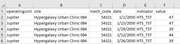
By opening up in Excel and inspecting it, we can see that the contents are tidy - there are 6 columns and 27 rows. The data appear to be recording monthly testing (HTS_TST) at a specific site by a specific mechanism and there are no missing values.
Now that we have reviewed the data, we can import into R. The base R
function to read in data is read.table(), which “reads a file in table
format and creates a data frame from it.” Instead of using base R, we
are going to take advantage of readr from the tidyverse. In R for Data
Science, Wickham and Grolemund explain:
Compared to read.table and its derivatives, readr functions are: 1. ~ 10 times faster 2. Return tibbles 3. Have more intuitive defaults. No row names, no strings as factors.
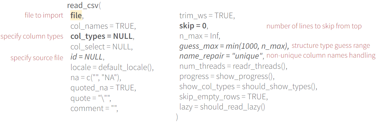
Let’s give read_csv(), “a special [case] of the more general
read_demin() a go. We just need to provide the file path from our
working directory to the file and pass that into the first parameter
(file) in read_csv(). With R, if you are working on a PC, you will
need to change the backslashes (”\”) in your file path to forward slashes
(“/”). (The data for this session can be found
here).
read_csv("simple.csv")
## Rows: 27 Columns: 6
## -- Column specification -------------------------------------------------------------------------
## Delimiter: ","
## chr  (3): operatingunit, site, indicator
## dbl  (2): mech_code, value
## date (1): date
##
## i Use `spec()` to retrieve the full column specification for this data.
## i Specify the column types or set `show_col_types = FALSE` to quiet this message.

## # A tibble: 27 x 6
##    operatingunit site                         mech_code date       indicator value
##    <chr>         <chr>                            <dbl> <date>     <chr>     <dbl>
##  1 Jupiter       Hypergalaxy Urban Clinic 084     54321 2050-01-01 HTS_TST      47
##  2 Jupiter       Hypergalaxy Urban Clinic 084     54321 2050-01-15 HTS_TST      47
##  3 Jupiter       Hypergalaxy Urban Clinic 084     54321 2050-01-29 HTS_TST      29
##  4 Jupiter       Hypergalaxy Urban Clinic 084     54321 2050-02-12 HTS_TST      44
##  5 Jupiter       Hypergalaxy Urban Clinic 084     54321 2050-02-26 HTS_TST      39
##  6 Jupiter       Hypergalaxy Urban Clinic 084     54321 2050-03-12 HTS_TST      36
##  7 Jupiter       Hypergalaxy Urban Clinic 084     54321 2050-03-26 HTS_TST      42
##  8 Jupiter       Hypergalaxy Urban Clinic 084     54321 2050-04-09 HTS_TST      25
##  9 Jupiter       Hypergalaxy Urban Clinic 084     54321 2050-04-23 HTS_TST      39
## 10 Jupiter       Hypergalaxy Urban Clinic 084     54321 2050-05-07 HTS_TST      41
## # ... with 17 more rows
The output displayed in the Console provide us some useful information
about the file. We can see the deliminter here was a comma, which we
already knew because it was a csv file. If we had used read_delim, the
function would have guessed the deliminter and displayed it here. The
next set of information in the output shows each of the columns and what
their column type is. For example, we can see operatingunit is being
read in as a chr or character and value is being read in as dbl or
double/numeric. And then lastly, we can see that read_csv() provides a
tibble back from what it read in (as well as it’s size 27 x 6).
We simply read in the file, but didn’t save it anywhere so it will show up in our Console, but not appear in the Environment to use later. If we did want to use this data, we would need to assign it to an object.
df_months <- read_csv("simple.csv")
## Rows: 27 Columns: 6
## -- Column specification -------------------------------------------------------------------------
## Delimiter: ","
## chr  (3): operatingunit, site, indicator
## dbl  (2): mech_code, value
## date (1): date
##
## i Use `spec()` to retrieve the full column specification for this data.
## i Specify the column types or set `show_col_types = FALSE` to quiet this message.
Export
The readr package is also equipt with functions to let us export the
data that we have read in (and presumability munged or modeled). We can
use write_csv to save the data.
write_csv(df_months, "simple_out.csv", na = "")
The last parameter in the function about, na = "", allows us to tell R
how to store missing values in the output. In this call, missing cells
will appear as blank cells in the csv output.
Diving into the parameters
There are a number of options or parameters for read_csv() that we can
inspect. We won’t go through them all, but it’s useful to highlight a
few of the ones you may use more frequently. These parameters are
mimicked in other import functions, so once you have these down, you can
apply them in the different packages/functions as you need.
It’s important to be aware of the different options as it can make your life much easier when you are faced with a problematic file to import in the future.
Parsing
Importing with readr is pretty smart, but it’s not always perfect.
Usually it does a pretty good job identifying the correct column types
(i.e. is it a date? character? logical? double?), but you can actually
provide the precise column type to the col_types parameter as an
option. Here are the different column times you can pass in:
- c = character
- i = integer
- n = number
- d = double
- l = logical
- f = factor
- D = date
- T = date time
- t = time
- ? = guess
- _ or - = skip
I’m not doing readr’s ability to guess justitice, so I would highly
recommend reading the parsing section in Chapter 11 of
R4DS.
I typically see an issue when there are thousands of lines in a column
that are missing and then there are values at the bottom. We can
replicate this by forcing read_csv() to only guess base on the first.
Let’s look at the missing.csv dataset, which has many of the value
rows missing, and just guess based on the first few lines.
read_csv("missing.csv", guess_max = 5)
## Warning: One or more parsing issues, see `problems()` for details

## Rows: 27 Columns: 6
## -- Column specification -------------------------------------------------------------------------
## Delimiter: ","
## chr  (3): operatingunit, site, indicator
## dbl  (1): mech_code
## lgl  (1): value
## date (1): date
##
## i Use `spec()` to retrieve the full column specification for this data.
## i Specify the column types or set `show_col_types = FALSE` to quiet this message.

## # A tibble: 27 x 6
##    operatingunit site                         mech_code date       indicator value
##    <chr>         <chr>                            <dbl> <date>     <chr>     <lgl>
##  1 Jupiter       Hypergalaxy Urban Clinic 084     54321 2050-01-01 HTS_TST   NA
##  2 Jupiter       Hypergalaxy Urban Clinic 084     54321 2050-01-15 HTS_TST   NA
##  3 Jupiter       Hypergalaxy Urban Clinic 084     54321 2050-01-29 HTS_TST   NA
##  4 Jupiter       Hypergalaxy Urban Clinic 084     54321 2050-02-12 HTS_TST   NA
##  5 Jupiter       Hypergalaxy Urban Clinic 084     54321 2050-02-26 HTS_TST   NA
##  6 Jupiter       Hypergalaxy Urban Clinic 084     54321 2050-03-12 HTS_TST   NA
##  7 Jupiter       Hypergalaxy Urban Clinic 084     54321 2050-03-26 HTS_TST   NA
##  8 Jupiter       Hypergalaxy Urban Clinic 084     54321 2050-04-09 HTS_TST   NA
##  9 Jupiter       Hypergalaxy Urban Clinic 084     54321 2050-04-23 HTS_TST   NA
## 10 Jupiter       Hypergalaxy Urban Clinic 084     54321 2050-05-07 HTS_TST   NA
## # ... with 17 more rows
readr::problems()
We can see that if we just use the first 5 lines to guess what the
column type is, it expected value to be a logical, when in fact there
are numeric values in the column, which we can see when we print out the
errors.
Let’s take a look at another example of guessing and column types before
we get in the resolution. If we look at back our df_months, we can see
that mech_code was read in as a double. Technically yes, mech_code
is comprised of digits, but it not a value we ever want to sum or use as
a filter (i.e. filter where mech_code is greater than 12000).
str(df_months)
## spec_tbl_df [27 x 6] (S3: spec_tbl_df/tbl_df/tbl/data.frame)
##  $ operatingunit: chr [1:27] "Jupiter" "Jupiter" "Jupiter" "Jupiter" ...
##  $ site         : chr [1:27] "Hypergalaxy Urban Clinic 084" "Hypergalaxy Urban Clinic 084" "Hypergalaxy Urban Clinic 084" "Hypergalaxy Urban Clinic 084" ...
##  $ mech_code    : num [1:27] 54321 54321 54321 54321 54321 ...
##  $ date         : Date[1:27], format: "2050-01-01" "2050-01-15" "2050-01-29" ...
##  $ indicator    : chr [1:27] "HTS_TST" "HTS_TST" "HTS_TST" "HTS_TST" ...
##  $ value        : num [1:27] 47 47 29 44 39 36 42 25 39 41 ...
##  - attr(*, "spec")=
##   .. cols(
##   ..   operatingunit = col_character(),
##   ..   site = col_character(),
##   ..   mech_code = col_double(),
##   ..   date = col_date(format = ""),
##   ..   indicator = col_character(),
##   ..   value = col_double()
##   .. )
##  - attr(*, "problems")=<externalptr>
We can change the column type to avoid any errors with using it in the
dataset and allow us to take advantage of tidyselect statements using
where(is.double), which should just specify your targets, results, and
cumulative (assuming we also change fiscal_year in the MSD to be
stored as an integer)). We can specify column types by passing a list
into col_types to tell it how you want the column read in. Let’s
adjust mech_code to be a character (“c” or col_character).
 read_csv("simple.csv",
          col_types = cols(mech_code = "c"))
## # A tibble: 27 x 6
##    operatingunit site                         mech_code date       indicator value
##    <chr>         <chr>                        <chr>     <date>     <chr>     <dbl>
##  1 Jupiter       Hypergalaxy Urban Clinic 084 54321     2050-01-01 HTS_TST      47
##  2 Jupiter       Hypergalaxy Urban Clinic 084 54321     2050-01-15 HTS_TST      47
##  3 Jupiter       Hypergalaxy Urban Clinic 084 54321     2050-01-29 HTS_TST      29
##  4 Jupiter       Hypergalaxy Urban Clinic 084 54321     2050-02-12 HTS_TST      44
##  5 Jupiter       Hypergalaxy Urban Clinic 084 54321     2050-02-26 HTS_TST      39
##  6 Jupiter       Hypergalaxy Urban Clinic 084 54321     2050-03-12 HTS_TST      36
##  7 Jupiter       Hypergalaxy Urban Clinic 084 54321     2050-03-26 HTS_TST      42
##  8 Jupiter       Hypergalaxy Urban Clinic 084 54321     2050-04-09 HTS_TST      25
##  9 Jupiter       Hypergalaxy Urban Clinic 084 54321     2050-04-23 HTS_TST      39
## 10 Jupiter       Hypergalaxy Urban Clinic 084 54321     2050-05-07 HTS_TST      41
## # ... with 17 more rows
Sometimes the best strategy when there are issues is to read in all the data as characters and then diagnose when in R. Rather than specify each column, you can define a default.
 read_csv("simple.csv",
          col_types = cols(.default = "c"))
## # A tibble: 27 x 6
##    operatingunit site                         mech_code date       indicator value
##    <chr>         <chr>                        <chr>     <chr>      <chr>     <chr>
##  1 Jupiter       Hypergalaxy Urban Clinic 084 54321     2050-01-01 HTS_TST   47
##  2 Jupiter       Hypergalaxy Urban Clinic 084 54321     2050-01-15 HTS_TST   47
##  3 Jupiter       Hypergalaxy Urban Clinic 084 54321     2050-01-29 HTS_TST   29
##  4 Jupiter       Hypergalaxy Urban Clinic 084 54321     2050-02-12 HTS_TST   44
##  5 Jupiter       Hypergalaxy Urban Clinic 084 54321     2050-02-26 HTS_TST   39
##  6 Jupiter       Hypergalaxy Urban Clinic 084 54321     2050-03-12 HTS_TST   36
##  7 Jupiter       Hypergalaxy Urban Clinic 084 54321     2050-03-26 HTS_TST   42
##  8 Jupiter       Hypergalaxy Urban Clinic 084 54321     2050-04-09 HTS_TST   25
##  9 Jupiter       Hypergalaxy Urban Clinic 084 54321     2050-04-23 HTS_TST   39
## 10 Jupiter       Hypergalaxy Urban Clinic 084 54321     2050-05-07 HTS_TST   41
## # ... with 17 more rows
Different packages and functions
So far, we’ve justed used readr to read in and write csv files. This
package can usually take us pretty far, but we can get data in a variety
of formats and sizes. So let’s look at a table of some other functions
and when we should use them over read_csv.
| package | function | description |
|---|---|---|
| readr | read_csv() | read in small/medium sized csv |
| readr | read_tsv() | read in small/medium sized tsv |
| readxl | read_excel() | read in an Excel file |
| googlesheets4 | read_sheet() | read small Google Sheet |
| googlesheets4 | range_speedread() | read large Google Sheet |
| data.table | fread() | read in large csv very fast |
| vroom | vroom() | read in large csv fast |
| haven | read_dta() | read in SAS/Stata/SPSS file |
| gophr | read_msd() | read in MER Structured Dataset/Genie output |
| tameDP | tame_dp() | read in PEPFAR Data Pack |
With read_excel(), the set up is pretty similar to read_csv, but
allows you to read in an Excel file. The key here is you typically want
to tell it what sheet to read in (sheet) or you can specify a range
(range). If you want to read in multiple sheets, you can take
advantage of the purrr::map_dfr() to iterate the import function over
all the tabs you’re interested in.
Let’s apply the ability to read in a specific sheet and take advantage
of something else we didn’t disuss earlier: the ability to skip rows.
We’ll look at the hfr.xlsx file, which has High Frequency Reporting
data (monthly data at the site level). We can use
readxl::excel_sheets() to identify the sheet in the workbook first.
excel_sheets("hfr.xlsx")
## [1] "meta" "HFR" "HFR Eridanus"
If we had opened the file first, we would have seen that the first row
contained human readable headers, not machine readable ones, which are
actually found on line 2. We can skip the first row and start reading in
from the second by providing the parameter skip = 1.
read_excel("hfr.xlsx", sheet = "HFR", skip = 1)
## # A tibble: 10 x 41
##    date                orgunit     orgunituid mech_code partner operatingunit psnu  hts_tst.u15.f
##    <dttm>              <chr>       <chr>          <dbl> <chr>   <chr>         <chr>         <dbl>
##  1 2050-01-01 00:00:00 Compact St~ RsbEDh3xi~     54321 Capric~ Jupiter       Naiad            17
##  2 2050-01-01 00:00:00 Neutrino U~ ZxF8BzC1U~     54321 Capric~ Jupiter       Naiad             9
##  3 2050-01-01 00:00:00 Moon Urban~ JnEgwmjsp~     54321 Capric~ Jupiter       Naiad             8
##  4 2050-01-01 00:00:00 Limb Darke~ TIqicPkbt~     54321 Capric~ Jupiter       Naiad            15
##  5 2050-01-01 00:00:00 Galactic N~ BRXw9Etn2~     54321 Capric~ Jupiter       Naiad            15
##  6 2050-01-01 00:00:00 Galactic N~ jmpRaM01S~     54321 Capric~ Jupiter       Naiad            18
##  7 2050-01-01 00:00:00 Hypergalax~ cQrI4UqvH~     54321 Capric~ Jupiter       Naiad            16
##  8 2050-01-01 00:00:00 Vernal Equ~ MNEI2PZqp~     54321 Capric~ Jupiter       Naiad             6
##  9 2050-01-01 00:00:00 Atmosphere~ cYyfQtNuF~     54321 Capric~ Jupiter       Naiad             8
## 10 2050-01-01 00:00:00 Meteor Hea~ kPw18xehd~     54321 Capric~ Jupiter       Naiad             7
## # ... with 33 more variables: hts_tst.u15.m <dbl>, hts_tst.o15.f <dbl>, hts_tst.o15.m <dbl>,
## #   hts_tst_pos.u15.f <dbl>, hts_tst_pos.u15.m <dbl>, hts_tst_pos.o15.f <dbl>,
## #   hts_tst_pos.o15.m <dbl>, tx_new.u15.f <lgl>, tx_new.u15.m <lgl>, tx_new.o15.f <lgl>,
## #   tx_new.o15.m <lgl>, vmmc_circ.u15.m <lgl>, vmmc_circ.o15.m <lgl>, prep_new.u15.f <lgl>,
## #   prep_new.u15.m <lgl>, prep_new.o15.f <lgl>, prep_new.o15.m <lgl>, tx_curr.u15.f <lgl>,
## #   tx_curr.u15.m <lgl>, tx_curr.o15.f <lgl>, tx_curr.o15.m <lgl>, tx_mmd.u15.f.u3mo <lgl>,
## #   tx_mmd.u15.m.u3mo <lgl>, tx_mmd.o15.f.u3mo <lgl>, tx_mmd.o15.m.u3mo <lgl>, ...
We can iterate over the sheets and combine them into one data frame
using purrr::map_dfr(). We can use the same function, but provide both
tabs to apply it to, pulling from the excel_sheets() function above
(there is a meta tab we also need to drop).
excel_sheets("hfr.xlsx") %>%
  str_subset("HFR") %>% #identify any sheets that contains "HFR"
  map_dfr(.f = ~read_excel("hfr.xlsx",
                                  sheet = .x,
                                  skip = 1))
## # A tibble: 20 x 41
##    date                orgunit     orgunituid mech_code partner operatingunit psnu  hts_tst.u15.f
##    <dttm>              <chr>       <chr>          <dbl> <chr>   <chr>         <chr>         <dbl>
##  1 2050-01-01 00:00:00 Compact St~ RsbEDh3xi~     54321 Capric~ Jupiter       Naiad            17
##  2 2050-01-01 00:00:00 Neutrino U~ ZxF8BzC1U~     54321 Capric~ Jupiter       Naiad             9
##  3 2050-01-01 00:00:00 Moon Urban~ JnEgwmjsp~     54321 Capric~ Jupiter       Naiad             8
##  4 2050-01-01 00:00:00 Limb Darke~ TIqicPkbt~     54321 Capric~ Jupiter       Naiad            15
##  5 2050-01-01 00:00:00 Galactic N~ BRXw9Etn2~     54321 Capric~ Jupiter       Naiad            15
##  6 2050-01-01 00:00:00 Galactic N~ jmpRaM01S~     54321 Capric~ Jupiter       Naiad            18
##  7 2050-01-01 00:00:00 Hypergalax~ cQrI4UqvH~     54321 Capric~ Jupiter       Naiad            16
##  8 2050-01-01 00:00:00 Vernal Equ~ MNEI2PZqp~     54321 Capric~ Jupiter       Naiad             6
##  9 2050-01-01 00:00:00 Atmosphere~ cYyfQtNuF~     54321 Capric~ Jupiter       Naiad             8
## 10 2050-01-01 00:00:00 Meteor Hea~ kPw18xehd~     54321 Capric~ Jupiter       Naiad             7
## 11 2050-01-01 00:00:00 Ubv Photom~ mJdHS2EZx~     54320 Eridan~ Jupiter       Hima~            10
## 12 2050-01-01 00:00:00 Astronomic~ qSbfXPBZz~     54320 Eridan~ Jupiter       Hima~            11
## 13 2050-01-01 00:00:00 Color Inde~ gNmf3QcZy~     54320 Eridan~ Jupiter       Hima~             5
## 14 2050-01-01 00:00:00 Brown Dwar~ Q3SkzF0Wt~     54320 Eridan~ Jupiter       Hima~            15
## 15 2050-01-01 00:00:00 Terminator~ S09aZ2Obk~     54320 Eridan~ Jupiter       Hima~            18
## 16 2050-01-01 00:00:00 Galilean M~ aEPjswAl3~     54320 Eridan~ Jupiter       Hima~             6
## 17 2050-01-01 00:00:00 Planetary ~ Hzv9TKsfe~     54320 Eridan~ Jupiter       Hima~             8
## 18 2050-01-01 00:00:00 Albedo Fea~ CwYUZehsF~     54320 Eridan~ Jupiter       Hima~             6
## 19 2050-01-01 00:00:00 Celestial ~ YDI1CUz9g~     54320 Eridan~ Jupiter       Hima~             5
## 20 2050-01-01 00:00:00 Irregular ~ tyRZiS24b~     54320 Eridan~ Jupiter       Hima~             4
## # ... with 33 more variables: hts_tst.u15.m <dbl>, hts_tst.o15.f <dbl>, hts_tst.o15.m <dbl>,
## #   hts_tst_pos.u15.f <dbl>, hts_tst_pos.u15.m <dbl>, hts_tst_pos.o15.f <dbl>,
## #   hts_tst_pos.o15.m <dbl>, tx_new.u15.f <lgl>, tx_new.u15.m <lgl>, tx_new.o15.f <lgl>,
## #   tx_new.o15.m <lgl>, vmmc_circ.u15.m <lgl>, vmmc_circ.o15.m <lgl>, prep_new.u15.f <lgl>,
## #   prep_new.u15.m <lgl>, prep_new.o15.f <lgl>, prep_new.o15.m <lgl>, tx_curr.u15.f <lgl>,
## #   tx_curr.u15.m <lgl>, tx_curr.o15.f <lgl>, tx_curr.o15.m <lgl>, tx_mmd.u15.f.u3mo <lgl>,
## #   tx_mmd.u15.m.u3mo <lgl>, tx_mmd.o15.f.u3mo <lgl>, tx_mmd.o15.m.u3mo <lgl>, ...
Since we work in the GSuite space, we can also take advantage of
directly accessing files stored in GDrive using the googlesheets4 (and
googledrive) package. You will need to authenticate your session each
time (check out the credential management vignette in
glamr
to learn how to store your USAID email for this purpose to make things
easier). The other difference is that you will need to provide the
function with the file id rather than a file path on a local machine.
gs4_auth() #only need to authenticate once per session
read_sheet(as_sheets_id("1B_DcG1WqZv6xo_eBBye-Q31tMGq_DjCBcjlWs3xINOw"))
## √ Reading from "simple_gs".

## √ Range 'simple.csv'.

## # A tibble: 27 x 6
##    operatingunit site                         mech_code date                indicator value
##    <chr>         <chr>                            <dbl> <dttm>              <chr>     <dbl>
##  1 Jupiter       Hypergalaxy Urban Clinic 084     54321 2050-01-01 00:00:00 HTS_TST      47
##  2 Jupiter       Hypergalaxy Urban Clinic 084     54321 2050-01-15 00:00:00 HTS_TST      47
##  3 Jupiter       Hypergalaxy Urban Clinic 084     54321 2050-01-29 00:00:00 HTS_TST      29
##  4 Jupiter       Hypergalaxy Urban Clinic 084     54321 2050-02-12 00:00:00 HTS_TST      44
##  5 Jupiter       Hypergalaxy Urban Clinic 084     54321 2050-02-26 00:00:00 HTS_TST      39
##  6 Jupiter       Hypergalaxy Urban Clinic 084     54321 2050-03-12 00:00:00 HTS_TST      36
##  7 Jupiter       Hypergalaxy Urban Clinic 084     54321 2050-03-26 00:00:00 HTS_TST      42
##  8 Jupiter       Hypergalaxy Urban Clinic 084     54321 2050-04-09 00:00:00 HTS_TST      25
##  9 Jupiter       Hypergalaxy Urban Clinic 084     54321 2050-04-23 00:00:00 HTS_TST      39
## 10 Jupiter       Hypergalaxy Urban Clinic 084     54321 2050-05-07 00:00:00 HTS_TST      41
## # ... with 17 more rows
Using vroom() is a pretty powerful tool to read in large datasets,
similar to fread(), but it is within the tidyverse. It’s also nice
because you can pass in multiple files to the same vroom statement and
it will read them in and store them as one tibble.
The last two functions are specific to PEPFAR, working with a MSD/Genie
file or a Data Pack and are pretty straight forward. The benefit of
using read_msd() over vroom() for a MSD/Genie file is that you are
returned with the correct structure for every column (and it cleans up
some of the extra genie files).
Homework
Problem: Using what you’ve learned, import in all the data from the HIV estimates to create a tidy dataset.
- Data do not start on the first row
- Columns are not uniquely named and have special character
- There are multiple tabs (hint: purrr::map_dfr)
- Missing values are written as “…”
- Values cells often contain characters (eg “<”) and thousand separators are spaces
- Upper and lower bounds should be separate columns
Originally sourced from here.
Homework solution
library(janitor)

xl_path <- "unaids_more_messy.xlsx"

excel_sheets(xl_path) %>%
  map_dfr(~read_excel(xl_path,
                      sheet = .x,
                      na = "...",
                      skip = 4,
                      col_types = "text",
                      .name_repair = janitor::make_clean_names)) %>%
  rename(year = x,
         iso = country,
         country = country_2,
         prev_adults_pct = percent_prevalence_adults,
         plhiv_adults =  estimated_plhiv_adults) %>%
  mutate(across(matches("plhiv"), ~ str_remove_all(. ," ")),
         across(matches("prev|percent|plhiv"), ~ str_remove_all(., "<")),
         across(.fns = ~ na_if(., "...,..."))) %>%
  separate(percent_prevalence_bounds, c("prev_lower", "prev_upper"), sep = ",") %>%
  separate(estimated_plhiv_bounds, c("plhiv_lower", "plhiv_upper"), sep = ",") %>%
  mutate(across(matches("prev|plhiv"), as.numeric))
## # A tibble: 172 x 9
##    year  iso   country prev_adults_pct prev_lower prev_upper plhiv_adults plhiv_lower plhiv_upper
##    <chr> <chr> <chr>             <dbl>      <dbl>      <dbl>        <dbl>       <dbl>       <dbl>
##  1 2020  AFG   Afghan~             0.1        0.1        0.2        11000        4500       41000
##  2 2020  AUS   Austra~             0.1        0.1        0.1        30000       24000       33000
##  3 2020  BGD   Bangla~            NA         NA         NA             NA          NA          NA
##  4 2020  BTN   Bhutan              0.2        0.1        0.5         1300         500        3000
##  5 2020  BRN   Brunei~            NA         NA         NA             NA          NA          NA
##  6 2020  KHM   Cambod~             0.5        0.5        0.6        72000       65000       80000
##  7 2020  CHN   China              NA         NA         NA             NA          NA          NA
##  8 2020  PRK   Democr~            NA         NA         NA             NA          NA          NA
##  9 2020  FJI   Fiji                0.2        0.1        0.4         1200         760        2400
## 10 2020  IND   India              NA         NA         NA             NA          NA          NA
## # ... with 162 more rows
Additional Resource
- Chapter 11 of R for Data Science for some really useful information both covered and not covered here.
- Check out the RStudio Import Cheat Sheet.
- Read through the packages pages, to check out all the functions, parameters, and examples/vignettes.
Next up
Now that we have a variety of tools for getting our data into R, we’ll spend our next couple of sessions talking about how to transform and clean it.