RBBS - 5 Introduction to the Tidyverse
2022-03-21 Tim Essam
corps rbbs r
For our R Building Blocks session today, we will focus on the
tidyverse. The technical portion of the session will focus on the
dplyr package for data wrangling.
Learning Objectives
- Learn what the tidyverse is and how it fits in the data science cycle
- Learn why the tidyverse is well suited for analytical work
- Learn how to use a few core data wrangling commands
Recording
USAID staff can use this link to access today’s recording (not available to external users).
Materials
Setup
For these sessions, we’ll be using RStudio which is an IDE, “Integrated development environment” that makes it easier to work with R. For help on getting setup and installing packages, please reference this guide.
What is the Tidyverse?
If you are an avid R user, you likely aware that are a many ways of accomplishing a task with R. Being an open source tool, R has many packages and approaches to tackling different types of analytically and data problems. This broad choice set can initially seem liberating. But, as you work your way through different packages, function inputs, data outputs, you may start to realize that the numerous ways of accomplishing a task can be detrimental. Having to switch back and forth between different package philosophies, grammar and data structures can become counterproductive. This leads us to the Tidyverse.
What is it? According to the Tidyverse webpage, “The tidyverse is an opinionated collection of R packages designed for data science. All packages share an underlying design philosophy, grammar, and data structures.” The packages fit together like puzzle pieces, with each package focusing on on part of the data science process. Before we dive into the process, let’s load the tidyverse and explore it a bit.
Let’s get started by installing install.packages("tidyverse") and
loading the library(tidyverse) to explore what packages are available
for use. Upon loading, you will notice that 8 core packages are imported
into the Rstudio session. Normally, when we use the library(package)
command, we expect a single package to be loaded. The tidyverse is an
exception to this in that it loads multiple packages when called.
library(tidyverse)
## Warning: package 'tidyverse' was built under R version 4.1.3

## -- Attaching packages --------------------------------------- tidyverse 1.3.1 --

## v ggplot2 3.3.5     v purrr   0.3.4
## v tibble  3.1.6     v dplyr   1.0.8
## v tidyr   1.2.0     v stringr 1.4.0
## v readr   2.1.2     v forcats 0.5.1

## -- Conflicts ------------------------------------------ tidyverse_conflicts() --
## x dplyr::filter() masks stats::filter()
## x dplyr::lag()    masks stats::lag()
So what do each of these packages do? Let’s review (paraphrased from Tidyverse webpage):
ggplot()- is a system for creating graphics, based on The Grammar of Graphics. It is the only tidyverse package that does not use the %>% (pipe) operator to chain together ggplot() lines.dplyr()- provides a grammar of data manipulation. The majority of commands are single data frame verbs (such asfilter,select,mutate,arrange). However, the joining commands (left_join,right_join,inner_join,full_join) rely on two data frames as inputs.tidyr()-provides a set of functions to help you in tidying data. Recall, that tidy data means each variable forms a column, each observation forms a row, and each cell is a measurement.readr()-provides a fast and friendly way to read in rectangular data (such as csv, tst, and fwf). It has numerous functions to flexibly parse many types of data found on the wild.purrr()- allows for replacing loops with cleaner code that is easier to write and read. It is an ideal tool for loading, joining and manipulating multiple MSDs at once, in a couple lines of code.tibble()- tibble is an opinionated and modern re-imagining of the data frame. Tibbles are data.frames that do less and complain more, to your benefit.stringr()- makes working with strings as easy as possibleforcats()- forcats provides a suite of useful tools that solve common problems with factors. We use forcats a ton for sorting columns to be plotted (fct_reorder())
# If you would like to explore the functions available in any of the tidyverse packages, use the following code chunk
ls('package:tibble')
##  [1] "%>%"                  "add_case"             "add_column"
##  [4] "add_row"              "as.tibble"            "as_data_frame"
##  [7] "as_tibble"            "as_tibble_col"        "as_tibble_row"
## [10] "char"                 "column_to_rownames"   "data_frame"
## [13] "data_frame_"          "deframe"              "enframe"
## [16] "frame_data"           "frame_matrix"         "glimpse"
## [19] "has_name"             "has_rownames"         "is.tibble"
## [22] "is_tibble"            "knit_print.trunc_mat" "lst"
## [25] "lst_"                 "new_tibble"           "num"
## [28] "obj_sum"              "remove_rownames"      "repair_names"
## [31] "rowid_to_column"      "rownames_to_column"   "set_char_opts"
## [34] "set_num_opts"         "set_tidy_names"       "size_sum"
## [37] "tbl_sum"              "tibble"               "tibble_"
## [40] "tibble_row"           "tidy_names"           "tribble"
## [43] "trunc_mat"            "type_sum"             "validate_tibble"
## [46] "view"
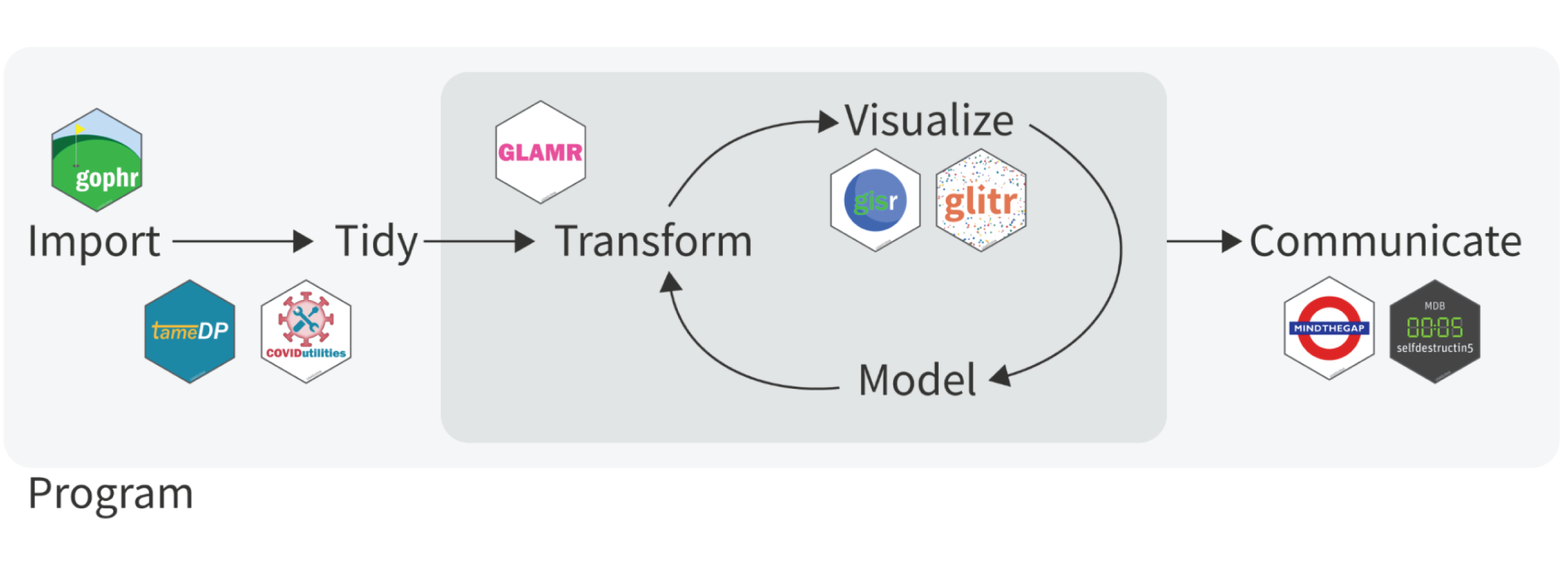
These packages work hand in hand to help you work your way through the
data science flow. In the graphic below, you can see where each package
fits. In the coming weeks, the coRps will delve into each package in a
bit more detail. For today, we’ll focus mainly on dplyr() and some
basics of data wrangling.
#

How do SI packages fit in this flow?
While readr() is an excellent choice for loading rectangular data
sets, the SI team tends to use the
vroom()
package because of its speed in loading large data sets, such as the
MSD. Moving to the tidy phase, the SI team has created a series of
packages (tameDP(), COVIDutilities(), and mindthegap()) to
facilitate the loading, tidying and preparing of different data streams.
glamr(), glitr(), and gisr() are largely focused on the transform,
visualization and modeling phase. Finally, mindthegap() and
selfdestructin5() are geared towards the communication aspect of the
flow.
Why use the Tidyverse?
When we sit down to work with a data set on a computer, three things need to happen. First, we need to know what we want to do with the data. If it has merged cells, we will need to unmerge them. If things are labelled inconsistently, we’ll need to relabel things in a standardized manner. If the data are wide when they should be long, we may have to change the physical layout of the rows and columns. To do all these things, we need to be able to communicate with a computer. If using Excel, we often do this through a series of points and clicks. If using R, Python, Stata or SAS, we can write computer code to tell a computer how something should be done. At the end of all this, we need to be able to get a computer to execute our code. The Tidyverse has been assembled with these steps in mind. It leverages action-oriented, descriptive functions to make it easier to express your data-related thoughts to the R program. As you get the hang of the syntax, you hopefully will find yourself with more time to think about what needs to be done and less time spent translating those tasks in code.
Consistency is one the primary reason we rely on the tidyverse for so much. What does this mean in terms of R code?
-
Function inputs - a data frame is always the first argument in a tidyverse function
-
Tidy data - a data frame is expected to be tidy when passed as an input
-
Tibble output - functions always return a tibble
-
Piping - the pipe (%>%) operator guides the flow of operations
When you put all these things together, the user experience tends to be much more pleasant. The predictability of what is required as an input (tidy data frame), what is expected as an output (tibble), layered on top of well named functions that can be easily chained together, leads to code that is easier to write, read and debug.
Let’s take a look at this visually using the hts data from the glitr
package. Imagine that we wanted to do the following:
-
filter the data to only rows where the
primepartneris Auriga and theperiodis FY50, -
group the data together by
indicatorandperiod_type, -
summarize the
valuefor each of those groups.
In base R, we would do something similar to the following:
#load the and review the data to ensure what we want to do is possible
library(glitr)
data(hts)
names(hts)
## [1] "operatingunit" "primepartner"  "indicator"     "modality"
## [5] "period"        "period_type"   "value"
str(hts)
## tibble [1,695 x 7] (S3: tbl_df/tbl/data.frame)
##  $ operatingunit: chr [1:1695] "Saturn" "Saturn" "Saturn" "Saturn" ...
##  $ primepartner : chr [1:1695] "Auriga" "Auriga" "Auriga" "Auriga" ...
##  $ indicator    : chr [1:1695] "HTS_TST" "HTS_TST" "HTS_TST" "HTS_TST" ...
##  $ modality     : chr [1:1695] "Index" "Index" "IndexMod" "IndexMod" ...
##  $ period       : chr [1:1695] "FY49" "FY50" "FY49" "FY50" ...
##  $ period_type  : chr [1:1695] "targets" "targets" "targets" "targets" ...
##  $ value        : num [1:1695] 3080 6880 890 780 6550 2170 870 2900 1200 1690 ...
aggregate(hts[(hts$primepartner == "Auriga") & (hts$period == "FY50"), ]$value,
  by = list(
    indicator = hts[(hts$primepartner == "Auriga") & (hts$period == "FY50"), ]$indicator,
    period_type = hts[(hts$primepartner == "Auriga") & (hts$period == "FY50"), ]$period_type
  ),
  FUN = sum, na.rm = TRUE
)
##     indicator period_type     x
## 1     HTS_TST  cumulative 11990
## 2 HTS_TST_POS  cumulative  1230
## 3     HTS_TST     targets 51970
## 4 HTS_TST_POS     targets  3430
The code chunk above does give use the desired outcome, but for a new (or even experienced) R user it is quite hard to follow along given all the nested operations. How could we do the same operation using tidyverse functions? The code chunk below executes the same operations. The pipe operator allows us to chain together three separate actions to create the desired output. The syntax is quite different from the base R approach. Tidyverse functions are named after action verbs which describe what should be done to an input. Even if a user doesn’t know R, they can probably deduce that the code below is filtering, grouping, and then summarizing something.
filter(hts, primepartner == "Auriga" & period == "FY50") %>%
  group_by(., indicator, period_type) %>%
  summarise(., total_results = sum(value, na.rm = T))
## `summarise()` has grouped output by 'indicator'. You can override using the
## `.groups` argument.

## # A tibble: 4 x 3
## # Groups:   indicator [2]
##   indicator   period_type total_results
##   <chr>       <chr>               <dbl>
## 1 HTS_TST     cumulative          11990
## 2 HTS_TST     targets             51970
## 3 HTS_TST_POS cumulative           1230
## 4 HTS_TST_POS targets              3430
Let’s take a look at the tidyverse approach line-by-line.
filter(hts, primepartner == "Auriga" & period == "FY50") %>%
In the first line, we are calling the filter() function to be used on
the data frame hts. The next part of the filter function
primepartner == "Auriga" & period == "FY50" provides the conditions by
which rows should be selected. In this case, we would like to keep all
rows where the primepartner is Auriga and the period is FY50. At the end
of the line, we use the %>% operator to pass the resulting tibble to
the next function.
group_by(., indicator, period_type) %>%
The group_by() function takes a data frame and converts it to a
grouped tbl where operations are then performed “by group”. Here, we ask
R to group the data by indicator and period type. Again, the %>% tells
R to pass the results to the next function.
summarise(., total_results = sum(value, na.rm = T))
Finally, the summarise() function creates a new column,
total_results, that is populated with the summarized amount of
value, by each of the groupings provided from the group_by() call –
indicator and period type.
How to use the Tidyverse
As reviewed above, the data science process has many phases across which
many of the tidyverse packages can be called on to help out. In the
remaining section, we will focus on the data wrangling portion using the
dplyr() package.
The dplyr() webpage describes the
package as a grammar of data manipulation built on a consistent set of
verbs that help you solve common data manipulation challenges. In total,
the packages has over 290 functions, but in your day to day work you
will likely be using some combination of 5 - 10 core functions. Let’s go
through some of these core functions, start with filter(), `
Filter
The filter() function is used to subset a data frame, based on logical
conditions that hold true for different rows. To be retained, a row must
produce a value of TRUE for all conditions. If a condition evaluates to
NA, the row will be dropped. The filter() command is a row focused
operation.
# The filter function will select rows based on their values. How could we go about filtering the data to only keep TBClinic testing modality for the primepartner Auriga?
hts %>%
  filter(modality == "TBClinic" & primepartner == "Auriga")
## # A tibble: 18 x 7
##    operatingunit primepartner indicator   modality period period_type value
##    <chr>         <chr>        <chr>       <chr>    <chr>  <chr>       <dbl>
##  1 Saturn        Auriga       HTS_TST     TBClinic FY49   targets      1380
##  2 Saturn        Auriga       HTS_TST     TBClinic FY50   targets       790
##  3 Saturn        Auriga       HTS_TST_POS TBClinic FY49   targets       500
##  4 Saturn        Auriga       HTS_TST_POS TBClinic FY50   targets       320
##  5 Saturn        Auriga       HTS_TST     TBClinic FY49Q1 results       800
##  6 Saturn        Auriga       HTS_TST     TBClinic FY50Q1 results       430
##  7 Saturn        Auriga       HTS_TST_POS TBClinic FY49Q1 results       180
##  8 Saturn        Auriga       HTS_TST_POS TBClinic FY50Q1 results       150
##  9 Saturn        Auriga       HTS_TST     TBClinic FY49Q2 results       860
## 10 Saturn        Auriga       HTS_TST_POS TBClinic FY49Q2 results       270
## 11 Saturn        Auriga       HTS_TST     TBClinic FY49Q3 results       910
## 12 Saturn        Auriga       HTS_TST_POS TBClinic FY49Q3 results       250
## 13 Saturn        Auriga       HTS_TST     TBClinic FY49Q4 results       660
## 14 Saturn        Auriga       HTS_TST_POS TBClinic FY49Q4 results       190
## 15 Saturn        Auriga       HTS_TST     TBClinic FY49   cumulative   1420
## 16 Saturn        Auriga       HTS_TST     TBClinic FY50   cumulative    430
## 17 Saturn        Auriga       HTS_TST_POS TBClinic FY49   cumulative    490
## 18 Saturn        Auriga       HTS_TST_POS TBClinic FY50   cumulative    150
Arrange
The arrange() function is used to order the rows of a data frame based
on the values of selected columns. By default, the function will return
an data frame ordered from smallest to largest (ascending). Use the
desc() option to sort in descending order. If multiple columns are
passed to the function, they are used to break ties in the values in the
preceding columns. The arrange() function is a row focused operation.
# Sort the data frame we just filtered above from highest to lowest value
hts %>%
  filter(modality == "TBClinic" & primepartner == "Auriga") %>%
  arrange(desc(value))
## # A tibble: 18 x 7
##    operatingunit primepartner indicator   modality period period_type value
##    <chr>         <chr>        <chr>       <chr>    <chr>  <chr>       <dbl>
##  1 Saturn        Auriga       HTS_TST     TBClinic FY49   cumulative   1420
##  2 Saturn        Auriga       HTS_TST     TBClinic FY49   targets      1380
##  3 Saturn        Auriga       HTS_TST     TBClinic FY49Q3 results       910
##  4 Saturn        Auriga       HTS_TST     TBClinic FY49Q2 results       860
##  5 Saturn        Auriga       HTS_TST     TBClinic FY49Q1 results       800
##  6 Saturn        Auriga       HTS_TST     TBClinic FY50   targets       790
##  7 Saturn        Auriga       HTS_TST     TBClinic FY49Q4 results       660
##  8 Saturn        Auriga       HTS_TST_POS TBClinic FY49   targets       500
##  9 Saturn        Auriga       HTS_TST_POS TBClinic FY49   cumulative    490
## 10 Saturn        Auriga       HTS_TST     TBClinic FY50Q1 results       430
## 11 Saturn        Auriga       HTS_TST     TBClinic FY50   cumulative    430
## 12 Saturn        Auriga       HTS_TST_POS TBClinic FY50   targets       320
## 13 Saturn        Auriga       HTS_TST_POS TBClinic FY49Q2 results       270
## 14 Saturn        Auriga       HTS_TST_POS TBClinic FY49Q3 results       250
## 15 Saturn        Auriga       HTS_TST_POS TBClinic FY49Q4 results       190
## 16 Saturn        Auriga       HTS_TST_POS TBClinic FY49Q1 results       180
## 17 Saturn        Auriga       HTS_TST_POS TBClinic FY50Q1 results       150
## 18 Saturn        Auriga       HTS_TST_POS TBClinic FY50   cumulative    150
Select
The select() function is used to subset columns based on the column
names or data type. It keeps or drops a column based on the input
parameters. There are many selection features (starts_with(),
ends_with(), matches(), and contains()) that can be applied to the
subset function. The select() function is a column oriented operation.
# Drop the operatingunit and primepartner from the dataframe
# The negation (!) component in the select call tells R to keep everything
# except the operatingunit and primepartner columns
hts %>%
  filter(modality == "TBClinic" & primepartner == "Auriga") %>%
  arrange(desc(value)) %>%
  select(!c(operatingunit, primepartner))
## # A tibble: 18 x 5
##    indicator   modality period period_type value
##    <chr>       <chr>    <chr>  <chr>       <dbl>
##  1 HTS_TST     TBClinic FY49   cumulative   1420
##  2 HTS_TST     TBClinic FY49   targets      1380
##  3 HTS_TST     TBClinic FY49Q3 results       910
##  4 HTS_TST     TBClinic FY49Q2 results       860
##  5 HTS_TST     TBClinic FY49Q1 results       800
##  6 HTS_TST     TBClinic FY50   targets       790
##  7 HTS_TST     TBClinic FY49Q4 results       660
##  8 HTS_TST_POS TBClinic FY49   targets       500
##  9 HTS_TST_POS TBClinic FY49   cumulative    490
## 10 HTS_TST     TBClinic FY50Q1 results       430
## 11 HTS_TST     TBClinic FY50   cumulative    430
## 12 HTS_TST_POS TBClinic FY50   targets       320
## 13 HTS_TST_POS TBClinic FY49Q2 results       270
## 14 HTS_TST_POS TBClinic FY49Q3 results       250
## 15 HTS_TST_POS TBClinic FY49Q4 results       190
## 16 HTS_TST_POS TBClinic FY49Q1 results       180
## 17 HTS_TST_POS TBClinic FY50Q1 results       150
## 18 HTS_TST_POS TBClinic FY50   cumulative    150
Mutate
The mutate() function adds new variables and preserves existing ones.
If you need to create a new column in your data based on the features of
other columns, mutate() is your friend. Be aware that if an existing
variable name is used in the mutate function, the resulting output will
overwrite existing variables of the same name. Mutate is a column
oriented operation.
hts %>%
  filter(modality == "TBClinic" & primepartner == "Auriga") %>%
  arrange(desc(value)) %>%
  select(!c(operatingunit, primepartner)) %>%
  group_by(indicator, period_type) %>%
  mutate(summed_value = sum(value, na.rm = T)) %>%
  ungroup()
## # A tibble: 18 x 6
##    indicator   modality period period_type value summed_value
##    <chr>       <chr>    <chr>  <chr>       <dbl>        <dbl>
##  1 HTS_TST     TBClinic FY49   cumulative   1420         1850
##  2 HTS_TST     TBClinic FY49   targets      1380         2170
##  3 HTS_TST     TBClinic FY49Q3 results       910         3660
##  4 HTS_TST     TBClinic FY49Q2 results       860         3660
##  5 HTS_TST     TBClinic FY49Q1 results       800         3660
##  6 HTS_TST     TBClinic FY50   targets       790         2170
##  7 HTS_TST     TBClinic FY49Q4 results       660         3660
##  8 HTS_TST_POS TBClinic FY49   targets       500          820
##  9 HTS_TST_POS TBClinic FY49   cumulative    490          640
## 10 HTS_TST     TBClinic FY50Q1 results       430         3660
## 11 HTS_TST     TBClinic FY50   cumulative    430         1850
## 12 HTS_TST_POS TBClinic FY50   targets       320          820
## 13 HTS_TST_POS TBClinic FY49Q2 results       270         1040
## 14 HTS_TST_POS TBClinic FY49Q3 results       250         1040
## 15 HTS_TST_POS TBClinic FY49Q4 results       190         1040
## 16 HTS_TST_POS TBClinic FY49Q1 results       180         1040
## 17 HTS_TST_POS TBClinic FY50Q1 results       150         1040
## 18 HTS_TST_POS TBClinic FY50   cumulative    150          640
Summarise
The summarise() function creates a new data frame. The new data frame
will have one (or more) rows for each combination of grouping variables.
If you are Stata user, the command is similar to the
collapse() function. If
using the function without a group_by() call, the output will have a
single row summarising all observations of the input.
hts %>%
  filter(modality == "TBClinic" & primepartner == "Auriga") %>%
  arrange(desc(value)) %>%
  select(!c(operatingunit, primepartner)) %>%
  group_by(indicator, period_type) %>%
  summarise(summed_value = sum(value, na.rm = T), .groups = "drop")
## # A tibble: 6 x 3
##   indicator   period_type summed_value
##   <chr>       <chr>              <dbl>
## 1 HTS_TST     cumulative          1850
## 2 HTS_TST     results             3660
## 3 HTS_TST     targets             2170
## 4 HTS_TST_POS cumulative           640
## 5 HTS_TST_POS results             1040
## 6 HTS_TST_POS targets              820
Practice at home
Problem: Use the dplyr verbs discussed to create a data frame that:
-
summarizes indicator results (not targets / cumulative)
-
for the only the first two quarters of FY49
-
for only index-based testing modalities
-
for the primeparter Auriga
#Homework solutions: Use the dplyr verbs discussed to create a data frame that summarizes indicator results for the first two quarters of FY49 for only index-based testing modalities for Auriga
hts %>%
  filter(period_type == "results" & str_detect(modality, "Index") & primepartner == "Auriga" & period %in% c("FY49Q1", "FY49Q2")) %>%
  group_by(indicator, modality) %>%
  summarise(results_q1_q2 = sum(value, na.rm = T), .groups = "drop")
## # A tibble: 4 x 3
##   indicator   modality results_q1_q2
##   <chr>       <chr>            <dbl>
## 1 HTS_TST     Index             7950
## 2 HTS_TST     IndexMod           300
## 3 HTS_TST_POS Index             1400
## 4 HTS_TST_POS IndexMod            10
# Another approach, filtering later on in the flow
hts %>%
  filter(modality %in% c("Index", "IndexMod"), period %in% c("FY49Q1", "FY49Q2")) %>%
  group_by(indicator, primepartner, period_type, modality) %>%
  summarise(results_q1_q2 = sum(value, na.rm = T), .groups = "drop") %>%
  arrange(primepartner) %>%
  filter(primepartner == "Auriga")
## # A tibble: 4 x 5
##   indicator   primepartner period_type modality results_q1_q2
##   <chr>       <chr>        <chr>       <chr>            <dbl>
## 1 HTS_TST     Auriga       results     Index             7950
## 2 HTS_TST     Auriga       results     IndexMod           300
## 3 HTS_TST_POS Auriga       results     Index             1400
## 4 HTS_TST_POS Auriga       results     IndexMod            10
Additional Resources
For more practice with dplyr, check out Allison Horst’s dplyr
tutorial.
For tutorials on Workflows for Data Analysis with R check out Julie Scholler’s training.
For a good guide on how to use the dplyr functions, see this
cheatsheet.
Next Up
This session, we covered some of the core data wrangling functions from
the dplyr() package. While this session offers a glimpse of how to do
basic data manipulation with the tidyverse, the following weeks will
cover different phases of the data science flow and the tidyverse
packages that can help you along each stage.